
Kimi K3's headline number is 2.8 trillion parameters. It is the least interesting number in the report.
The interesting part is that the architecture is organized around a question that has nothing to do with size: where is information failing to flow? The answer has three parts — along the sequence, along the depth, along the width — and each gets its own mechanism.
Same compute, roughly 2.5× the scaling efficiency of Kimi K2. That figure comes from the team's own fitted scaling-law curves rather than a third-party reproduction, so read it as their claim. But the mechanisms behind it are specific enough to argue with, which is what makes the report worth the time.
This is a close read of the Kimi K3 technical report (Moonshot AI), focused on its architecture section. We have written before about long-horizon agent design; this one sits further down the stack.
Three directions, not one number
Every layer in a transformer mixes information three ways. Across tokens, so position 900,000 can affect position 1. Across depth, so layer 90 can use what layer 3 noticed. Across channels, so features can recombine.
Most scaling work moves all three at once by making everything bigger. K3 separates them and gives each its own mechanism:
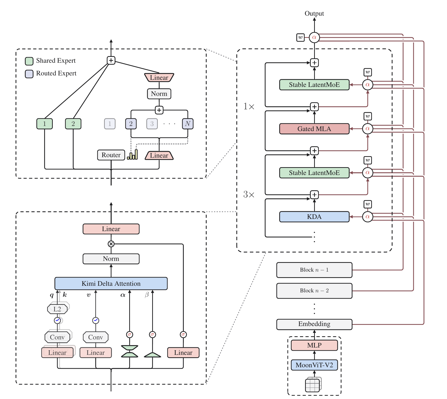
- Sequence — hybrid attention: three Kimi Delta Attention layers for every one Gated MLA layer.
- Depth — Attention Residuals: each layer attends over the outputs of all preceding layers instead of inheriting one accumulated state.
- Width — Stable LatentMoE: 896 routed experts, 16 awake per token.
The hidden dimension did not change at all. 7,168 in K2, 7,168 in K3. Whatever got bigger, it was not the width of a layer.
Sequence: three quarters of the layers stopped reading everything
Standard attention re-reads the whole prefix for every new token. At a million tokens, that bill is what breaks.
K3 splits the job. Three KDA layers keep a fixed-size running state — closer to taking notes than to re-reading the source — followed by one Gated MLA layer doing full global attention. The pattern repeats, with one extra MLA layer at the very end so the final layer always sees everything. Across 93 layers: 69 KDA, 24 MLA.
The fixed size is the whole point. The state does not grow with the sequence, so it cannot blow up. It is also lossy, which is why a full-attention layer appears every fourth layer to recover what the notes dropped.
Then a second-order effect. Because the recurrent state carries a decay — recent tokens are naturally more present than old ones — position information comes along for free. So K3 applies no positional encoding at all to its global-attention layers. No RoPE, nothing to rescale.
Which means extending to a million tokens required no positional-encoding surgery. None of the interpolation tricks the field has accumulated for context extension apply here, because there is no encoding to interpolate.
A lower bound that deleted a GPU code path
This is our favourite part of the report, and it is small enough to skim past.
The recurrent state forgets as it goes. Computing that efficiently in chunks requires dividing by the accumulated decay, and accumulated decay is a product of numbers below one. Let it run unchecked and you are dividing by something arbitrarily close to zero.
The previous generation handled this by splitting each chunk into 16-token tiles and working in log space. It worked, but the tiles on the diagonal still had to be evaluated position pair by position pair — a slow, special-cased path that could not use the tensor cores.
K3's fix is one line of parameterization. Bound the log-decay from below: each step may forget down to 0.67% of what it was holding, and no further.
Follow it through. With that bound, accumulated log-decay over a 16-token tile stays inside (−80, 0). The reciprocal is therefore under e80 ≈ 5.5 × 1034, comfortably within BF16's range of about 3.4 × 1038. Nothing overflows. So the diagonal tiles can use the same dense matrix multiplication as every other tile.
The special path is not optimized. It is gone.
Read the causality backwards and it gets better: the hardware's dynamic range determined the acceptable interval, which determined the constant, which determined that the activation had to be bounded below. The numerics chose the math, not the other way around.
Depth: from a relay race to a group chat
Ninety-three layers deep, the standard residual stream is a relay race. Layer 50 receives one accumulated state from layer 49. Whatever layers 1 through 48 individually noticed has been summed into that state and is no longer separable.
The paper's framing is that this is the same bottleneck an RNN has over time — and the field already solved that one, with attention. Attention Residuals apply the same fix to depth: each layer carries a learnable pseudo-query and attends over the outputs of all preceding layers, choosing what to read.
Done literally this costs quadratic compute in depth and, worse, keeps every layer's output alive in memory and on the wire under pipeline parallelism. So K3 uses the block variant: 93 layers partitioned into groups of twelve, summed within a group, full attention across groups. Overhead drops from per-layer to per-group, and the inference-time state stays bounded.
Width: 896 experts, 16 awake
Mixture-of-experts keeps a large pool and wakes a few per token. K2 chose 8 of 384. K3 chooses 16 of 896 — a sparsity of 56.
Growing the pool that far breaks two things, and the report is unusually direct about both.
Communication. In a conventional MoE, every selected expert receives the full-width token, so traffic scales with how many you select. LatentMoE decouples the two: routed experts work in a compact latent space at half the model width, while two full-width shared experts handle what every token needs. The pool can grow without the wire cost growing with it.
Stability. At this sparsity the routed branch becomes a chain of nearly four consecutive matrix multiplications, and activations explode. Two fixes: an RMSNorm between expert aggregation and the up-projection, and a new activation, SiTU-GLU, which caps both factors of a SwiGLU with a scaled tanh so neither can run away in low precision.
Balance. The third fix is the one worth stealing. Keeping roughly 900 experts evenly loaded means adjusting a per-expert bias every step. The standard method nudges each bias by a fixed increment in the direction of the error, which either oscillates or lags. K3 solves for it instead: run top-(k+1) rather than top-k, and the extra entry is the score a token demands for admission. With those cutoffs in hand, the load an expert receives under a candidate bias is monotone, so the bias that hits the target load is simply a quantile of the margins. One forward pass, no step size to tune.
At scale that quantile spans millions of values across every rank, so they estimate it from a histogram: each rank counts its bins, one all-reduce sums them, the quantile is read off the pooled counts. Counts add, so the estimate reflects the whole batch regardless of how tokens are sharded, at a cost of a few hundred bins per expert.
The bill comes due in the serving stack
None of this is free, and the honest part of the report is the infrastructure section, where the cost lands.
A fixed-size recurrent state is cheap to store and cheap to move, but it updates serially and it does not simply add. Both properties create work:
- Splitting a sequence across devices. Ordinary linear attention lets each device compute its local state from zero and sum the results. KDA applies a token-dependent transition to the incoming state, so summation is wrong. The fix decomposes each segment into a cumulative transition and a zero-start state — two quantities that do compose — and recovers each device's entry state with a prefix scan and one fixed-size all-gather.
- Reusing a prefix across requests. Half the caches are per-token pages, half are one fixed state per request, and a cache hit needs both restorable at the same boundary. Their answer is to decouple the granularities: hash at 512 tokens, allocate at 1024–6144, and checkpoint the recurrent state only at a sparse subset of hash endpoints.
- Speculative decoding. The state updates in place, so a rejected draft cannot be rolled back. They cache the projected inputs instead — far smaller than the state itself — and rebuild on chip.
The pattern across all three is the one from the decay bound, run in the other direction: the architecture chose a representation, and the representation dictated the systems work.
One habit the paper quietly drops
K3 is natively multimodal, and its vision encoder is trained from scratch with next-token prediction. No SigLIP initialization, no contrastive pre-training — which is the standard recipe, including in the team's own previous model.
The stated reason is not quality. It is stability: the contrastively initialized encoder showed persistently higher gradient norms with frequent spikes under joint optimization, while the from-scratch one stayed flat. Vision evaluations came out even.
That makes the finding sharper than a win would have been. If from-scratch had been better, you would call it a better recipe. It matched — so the claim is that at this scale, a step the field treats as mandatory is merely optional.
What this means if you run agents on these models
We build a multi-agent desktop client, so what we watch is whether a long-horizon run stays affordable, not what tops a leaderboard.
The number that matters is not the size of the context window; it is what a million tokens costs to serve. Three quarters of the layers carry a fixed-size state, so the cache that grows with the conversation is a quarter the size it would be in an all-attention model of the same depth. On BrowseComp the report puts K3 at 91.2% at roughly $2 per task — about half the cost of the nearest proprietary score, and an order of magnitude under the Claude models at maximum effort.
For an agent running hundreds of tool calls, that ratio decides whether a task is worth attempting at all. Architecture work that used to read as pure research now shows up directly in whether a long run is economically sane.
What we take from it
Two things, both transferable.
First, the framing. Where is information failing to flow? produces different work than how much bigger can we go? — and it decomposes, which is why three mechanisms could be developed and measured separately.
Second, the decay bound. A constraint that costs almost nothing in expressiveness removed an entire special-cased path from the kernel. Not a faster path — no path. That trade is available far more often than it gets taken, and it is only visible to people holding the math and the hardware at the same time.
The report and the weights are open on GitHub. The architecture section is eight pages and repays a careful read.